Create Pivot Table In Excel – Microsoft Excel is very useful software because of which we can do many hours of work in minutes. We can make the work very easy by applying formulas in Excel, if we want to find anything, we can find it with the help of formulas. You too must have used formulas in Excel at some point of time. The pivot table is the most used formula in Excel, so today in this article I will tell you how you can use pivot table.
In this article, we are going to see how to create pivot table in excel, Before that we know what is pivot table.
what is the use of pivot table in excel?
If we want to understand in simple language, then with the help of Pivot table formula, we can give a simple form to the biggest data, out of that we can make a table of some data.
By the way, this formula is used in many places, but in the biggest company, to give a simple form to the data of the sales and to find out from it where and how much sell has been sold, it is most commonly used for this.
How To Create Pivot Table In Excel ?
To use this formula, first of all, you must have Microsoft Office installed on your laptop or PC.
what is the first step for creating a pivot table?
To use it, first of all, you have to open the Excel software in your laptop or PC, if Microsoft Office is installed in your laptop, then you will see the icon of Excel in the laptop or PC, you have to click on it.

Step.2
Now you have to open the data on which you have to use the pivot table formula,Now you have to select the entire data, you can do this with the help of Carcer or you can also select the entire data by Crtl+A.

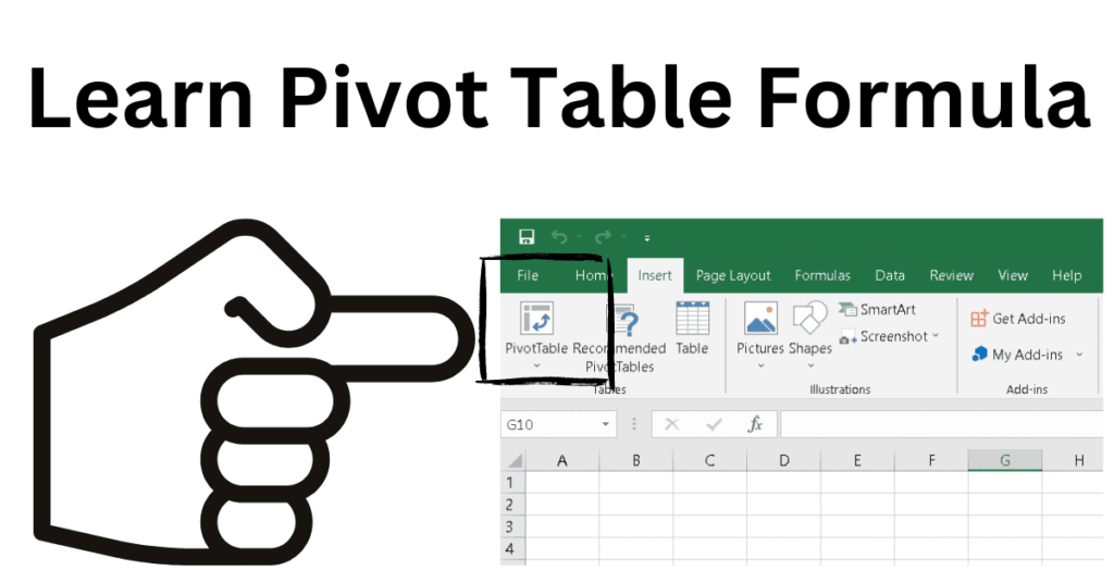
under which tab and in which function group will you find the option to insert a pivot table?
In the top menu bar of Excel, you will see the option of insert, you have to click on it, and there you will see the option of pivot table, simply you have to click on it Or you can open pivot table formula by the help of pivot table shortcut Ctrl+N+V.

Step. 4
After this a dialog box will open, and some options will appear in it.

Select A Table Or Range
In this option, the amount of data you have selected will be visible, you can set the range of this data according to you.
Choose Where You Want Pivot Table In Excel To Be Placed
New Worksheet – Whatever data you want to apply this formula, this formula will be prepared on a new Excel sheet.
Existing Worksheet – If you want to apply that formula in the same worksheet then click on it.
Step.5
After that, you have to click on OK, and you will see your pivot table, To the right of the table, you will see the option of data, Now your pivot table is ready, now you can use this data as you want.
Conclusion
In this article, we have told all the information about how to create Pivot Table in excel an easy way. If you like the information, then definitely share this article with your friends and family members, it can be helpful for them.
Read this also
How To Add Watermark In Excel 2024